Recurrent versus Disruption Risk

The distinction between disruptions and recurrent / continuous risks is commonly used by researchers and practitioners in supply chain management. But how should the differences be reflected in the supply chain planning process? Is it necessary to differentiate between the risk types here as well?

In 2007 Sunil Chopra et al. analyzed this question in depth.

Disruption vs. continuous risks

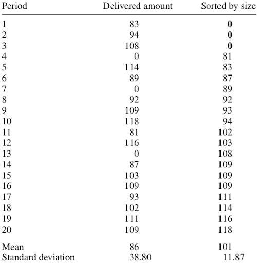
For simplicity sake the authors define a disruption as a supplier which does not deliver any product at all. Figure 1 shows an example delivery listing for 20 periods. In periods 4, 7 and 13 nothing has been delivered and so a disruption has happened.

As you can see the overall mean (including the disrupted periods) is 86 with a standard deviation of 39. But the third column highlights an important point: If you leave out the disrupted periods, the mean rises and the standard deviation drops to a third. As a result it should make a difference if a decision maker used one or the other mean / standard deviation to make his decision.

Figure 1: Exemplary Table containing Recurrent and Disruption Risks (Chopra et al., 2007)

Model

To test the effects of a differentiated versus a bundled view the authors develop a model. The focal company has two suppliers, one reliable and one unreliable (at risk of a disruption). The authors then analyze two cases: first, only recurrent risk and second, recurrent and disruption risks. Each with either a decision maker who views the risks bundled together or separately.
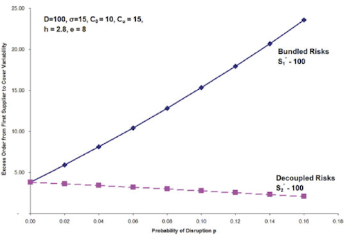
Figure 2 has a good graphic to show the implications of the different approaches with disruptions present. In a bundled view the excess order volume (y-axis, to prevent stock-outs) is increasing when the probability of the disruption increases. On the other hand, when the risks are decoupled the decision maker only focusses on the recurrent risk and the excess order even decreases with the probability of a disruption. The disruption risk is then mitigated by contingently using the more reliable supplier.

Figure 2: Comparison of Excess Orders for Decoupled and Non-Decoupled Risks (Chopra et al., 2007)

Implications

The authors conclude that:

Bundling of disruption and recurrent supply uncertainty results in an over (under) utilization of the low cost (reliable) supplier. The extent of over (under) utilization increases as the probability of disruption grows.

Furthermore:

Growth in supply risk from increased disruption probability is best mitigated by increased use of the reliable (though more expensive) supplier and decreased use of the cheaper but less reliable supplier. Growth in supply risk from increased recurrent uncertainty, however, is better served by increased use of the cheaper, though less reliable, supplier.

Conclusion

I liked the article a lot, since it focusses on one simple question: Is it bad to combine different types of risk. The conclusion: There will always be different risk sources or types which, as this article shows, have to be mitigated differently as well.